python machine-learning scikit-learn roc auc

Plotting the ROC curve for a multiclass problem

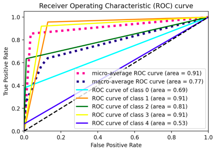
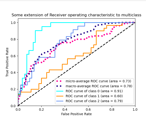
I am trying to apply the idea of sklearn ROC extension to multiclass to my dataset. My per-class ROC curve looks find of a straight line each, unline the sklearn's example showing curve's fluctuating.

I give an MWE below to show what I mean:

# all imports
import numpy as np
import matplotlib.pyplot as plt
from itertools import cycle
from sklearn import svm, datasets
from sklearn.metrics import roc_curve, auc
from sklearn.model_selection import train_test_split
from sklearn.preprocessing import label_binarize
from sklearn.datasets import  make_classification
from sklearn.ensemble import RandomForestClassifier
# dummy dataset
X, y = make_classification(10000, n_classes=5, n_informative=10, weights=[.04, .4, .12, .5, .04])
train, test, ytrain, ytest = train_test_split(X, y, test_size=.3, random_state=42)

# random forest model
model = RandomForestClassifier()
model.fit(train, ytrain)
yhat = model.predict(test)

The following function then plots the ROC curve:

def plot_roc_curve(y_test, y_pred):
  
  n_classes = len(np.unique(y_test))
  y_test = label_binarize(y_test, classes=np.arange(n_classes))
  y_pred = label_binarize(y_pred, classes=np.arange(n_classes))

  # Compute ROC curve and ROC area for each class
  fpr = dict()
  tpr = dict()
  roc_auc = dict()
  for i in range(n_classes):
    fpr[i], tpr[i], _ = roc_curve(y_test[:, i], y_pred[:, i])
    roc_auc[i] = auc(fpr[i], tpr[i])
  
  # Compute micro-average ROC curve and ROC area
  fpr["micro"], tpr["micro"], _ = roc_curve(y_test.ravel(), y_pred.ravel())
  roc_auc["micro"] = auc(fpr["micro"], tpr["micro"])

  # First aggregate all false positive rates
  all_fpr = np.unique(np.concatenate([fpr[i] for i in range(n_classes)]))

  # Then interpolate all ROC curves at this points
  mean_tpr = np.zeros_like(all_fpr)
  for i in range(n_classes):
    mean_tpr += np.interp(all_fpr, fpr[i], tpr[i])

  # Finally average it and compute AUC
  mean_tpr /= n_classes

  fpr["macro"] = all_fpr
  tpr["macro"] = mean_tpr
  roc_auc["macro"] = auc(fpr["macro"], tpr["macro"])

  # Plot all ROC curves
  #plt.figure(figsize=(10,5))
  plt.figure(dpi=600)
  lw = 2
  plt.plot(fpr["micro"], tpr["micro"],
    label="micro-average ROC curve (area = {0:0.2f})".format(roc_auc["micro"]),
    color="deeppink", linestyle=":", linewidth=4,)

  plt.plot(fpr["macro"], tpr["macro"],
    label="macro-average ROC curve (area = {0:0.2f})".format(roc_auc["macro"]),
    color="navy", linestyle=":", linewidth=4,)

  colors = cycle(["aqua", "darkorange", "darkgreen", "yellow", "blue"])
  for i, color in zip(range(n_classes), colors):
    plt.plot(fpr[i], tpr[i], color=color, lw=lw,
        label="ROC curve of class {0} (area = {1:0.2f})".format(i, roc_auc[i]),)

  plt.plot([0, 1], [0, 1], "k--", lw=lw)
  plt.xlim([0.0, 1.0])
  plt.ylim([0.0, 1.05])
  plt.xlabel("False Positive Rate")
  plt.ylabel("True Positive Rate")
  plt.title("Receiver Operating Characteristic (ROC) curve")
  plt.legend()

Output:

plot_roc_curve(ytest, yhat)

Kind of straight line bending once. I would like to see the model performance at different thresholds, not just one, a figure similar to sklearn's illustration for 3-classes shown below:

Solution

Point is that you're using predict() rather than predict_proba()/decision_function() to define your y_hat. This means - considering that the threshold vector is defined by the number of distinct values in y_hat (see here for reference), that you'll have few thresholds per class only on which tpr and fpr are computed (which in turn implies that your curves are evaluated at few points only).
Indeed, consider what the doc says to pass to y_scores in roc_curve(), either prob estimates or decision values. In the example from sklearn, decision values are used to compute the scores. Given that you're considering a RandomForestClassifier(), considering probability estimates in your y_hat should be the way to go.

What's the point then of label-binarizing the output? The standard definition for ROC is in terms of binary classification. To pass to a multiclass problem, you have to convert your problem into binary by using OneVsAll approach, so that you'll have n_class number of ROC curves. (Observe, indeed, that as SVC() handles multiclass problems in a OvO fashion by default, in the example they had to force to use OvA by applying OneVsRestClassifier constructor; with a RandomForestClassifier you don't have such problem as that's inherently multiclass, see here for reference). In these terms, once you switch to predict_proba() you'll see there's no much sense in label binarizing predictions.

 # all imports
 import numpy as np
 import matplotlib.pyplot as plt
 from itertools import cycle
 from sklearn import svm, datasets
 from sklearn.metrics import roc_curve, auc
 from sklearn.model_selection import train_test_split
 from sklearn.preprocessing import label_binarize
 from sklearn.datasets import  make_classification
 from sklearn.ensemble import RandomForestClassifier
 # dummy dataset
 X, y = make_classification(10000, n_classes=5, n_informative=10, weights=[.04, .4, .12, .5, .04])
 train, test, ytrain, ytest = train_test_split(X, y, test_size=.3, random_state=42)

 # random forest model
 model = RandomForestClassifier()
 model.fit(train, ytrain)
 yhat = model.predict_proba(test)

 def plot_roc_curve(y_test, y_pred):
     n_classes = len(np.unique(y_test))
     y_test = label_binarize(y_test, classes=np.arange(n_classes))

     # Compute ROC curve and ROC area for each class
     fpr = dict()
     tpr = dict()
     roc_auc = dict()
     thresholds = dict()
     for i in range(n_classes):
       fpr[i], tpr[i], thresholds[i] = roc_curve(y_test[:, i], y_pred[:, i], drop_intermediate=False)
     roc_auc[i] = auc(fpr[i], tpr[i])

     # Compute micro-average ROC curve and ROC area
     fpr["micro"], tpr["micro"], _ = roc_curve(y_test.ravel(), y_pred.ravel())
     roc_auc["micro"] = auc(fpr["micro"], tpr["micro"])

     # First aggregate all false positive rates
     all_fpr = np.unique(np.concatenate([fpr[i] for i in range(n_classes)]))

     # Then interpolate all ROC curves at this points
     mean_tpr = np.zeros_like(all_fpr)
     for i in range(n_classes):
       mean_tpr += np.interp(all_fpr, fpr[i], tpr[i])

     # Finally average it and compute AUC
     mean_tpr /= n_classes

     fpr["macro"] = all_fpr
     tpr["macro"] = mean_tpr
     roc_auc["macro"] = auc(fpr["macro"], tpr["macro"])

     # Plot all ROC curves
     #plt.figure(figsize=(10,5))
     plt.figure(dpi=600)
     lw = 2
     plt.plot(fpr["micro"], tpr["micro"],
     label="micro-average ROC curve (area = {0:0.2f})".format(roc_auc["micro"]),
     color="deeppink", linestyle=":", linewidth=4,)

     plt.plot(fpr["macro"], tpr["macro"],
     label="macro-average ROC curve (area = {0:0.2f})".format(roc_auc["macro"]),
     color="navy", linestyle=":", linewidth=4,)

     colors = cycle(["aqua", "darkorange", "darkgreen", "yellow", "blue"])
     for i, color in zip(range(n_classes), colors):
       plt.plot(fpr[i], tpr[i], color=color, lw=lw,
       label="ROC curve of class {0} (area = {1:0.2f})".format(i, roc_auc[i]),)

     plt.plot([0, 1], [0, 1], "k--", lw=lw)
     plt.xlim([0.0, 1.0])
     plt.ylim([0.0, 1.05])
     plt.xlabel("False Positive Rate")
     plt.ylabel("True Positive Rate")
     plt.title("Receiver Operating Characteristic (ROC) curve")
     plt.legend()

Eventually, consider that roc_curve() has also a drop_intermediate parameter meant for dropping suboptimal thresholds (it might be useful to know).