Patching a color gradient with respect to given angular data
I am trying to patch a color gradient of given angular data
Here is the data:
n = [263.6909 287.9987 262.1933 199.6890 128.5683 71.1718 34.6535 15.2568 6.2683 2.4868 0.9872 0.4063 0.1793 0.0876 0.0487 0.0315 0.0241 0.0221 0.0243 0.0319 0.0495 0.0895 0.1838 0.4174 1.0159 2.5605 6.4504 15.6740 35.5053  72.6566 130.6707 201.9328];

theta=0:(2*pi/32):(2*pi*(32-1)/32);
theta(theta>pi) = theta(theta>pi)-2*pi;
I use a patch command
figure
hold on
patch(cos(theta), sin(theta), n, 'EdgeColor', 'none');
quiver(0,0,-4.6492,-0.9099,0.5,'k','linewidth',3);
axis equal
** edit start 3/12/2024 **
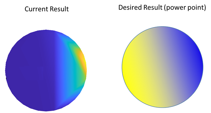
The gradient is suppose to be perpendicular to the line between the peak of the concentration and the opposite point along the rim (i.e, from $\theta(n_{max})$ and $\theta(n_{max}+\pi)).
There are two options I'm trying to apply:
1.Assuming that there is an exponential decaying gradient where the gradient patch decays from n_max to zero in the vertical direction.
- fitting a Gaussian to the data and use that with a corresponding theta which is segmented equally with respect to the location of the peak (i.e, one of the array point of theta is exactly where the peak is).
** edit end 3/12/2024 **
Here in the plot below is what I obtain, and what I wish to obtain
I highlight that the data is part of a dynamical simulation where the array n changes every iteration, and therefore the gradient slope, and direction, must be according to the given n
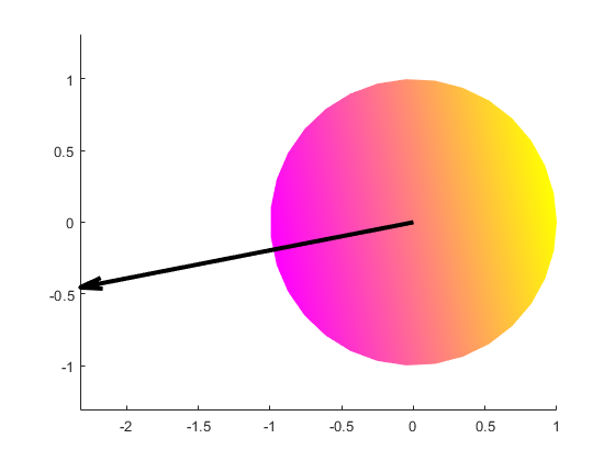
Your vector n is not smooth, and doesn't represent a parallel gradient to any vector direction. You can see this by just using plot(n), it aligns with the representation you get. This code shows how you can plot a gradient perpendicular to a given vector:
You can use atan2 to work out the direction of your vector aUV, and set the colour equal to cos(theta + aUV + pi/2), since you want to start drawing the colours offset by aUV from where you're drawing the circular patch and the additional pi/2 makes the gradient perpendicular.
% Some setup values
N = 32;        % Number of samples in array
U = -4.6492;   % X displacement of vector
V = -0.9099;   % Y displacement of vector
% Calculate circle drawing vectors
aUV = atan2(U,V);              % Angle of UV vector
theta = linspace(0,2*pi,N);    % Angle array for drawing patch
clr = cos(theta + aUV + pi/2); % Offset cyclic colour starting from aUV+pi/2
% Plot
figure(1); clf; hold on;
patch(cos(theta), sin(theta), clr, 'EdgeColor', 'none');
quiver(0,0,U,V,0.5,'k','linewidth',3);
axis equal; colormap spring
Output:
Edit with respect to question update...
If you do not have the angle or direction vector as an input we can determine it from the input n by
- Upsampling with piecewise cubic interpolation
- Finding the peak
- Plotting in a similar way to above
See the code comments for details
% Sort theta so that we can interpolate with it as the axis
[theta,idx] = sort(theta);
n = n(idx); % Match the order of points in 'n' with sorted theta
% Upsample 'n' using piecewise cubic interpolation
theta_i = linspace(theta(1),theta(end),1000);
n_i = interp1( theta, n, theta_i, 'pchip' );
% Find the index for the max value of 'n'
[n_max,idx] = max(n_i);
aUV = theta_i(idx);

% Offset cyclic colour starting from aUV
clr = cos(theta - aUV);

% Plotting... side by side of input curve with gradient for comparison
label = sprintf('\\theta=%.3f',aUV); % helper for legend labelling
figure(1); clf;

subplot(1,3,1); hold on;
plot(theta,n,'displayname','Input "n"');
plot(theta_i,n_i,'displayname','Upsampled "n"');
plot(aUV,n_max,'kx','displayname',['Peak "n" at ' label]);
legend('show','location','south');

subplot(1,3,2:3); hold on;
patch(cos(theta), sin(theta), clr, 'EdgeColor', 'none','displayname','gradient');
line( [-1,1]*cos(aUV), [-1,1]*sin(aUV), 'color', 'k', 'displayname', ['Ref line at ' label]);
axis equal; colormap parula; legend show
Result:
- In Matlab how to unpack a buffer of 12 bit values into an array of normalized float32
- How to use kmeans in python with Pearson correlation as distance measure, similar to MATLAB?
- How to test private methods using matlab.unittest?
- Variance in random Walk with Matlab
- Zero Padding, Discarding of Bits, and Adding Start and Stop Bits - MATLAB
- How to format the integer value with leading zeros in matlab?
- Variable number of left zeros in Matlab string
- Efficient and fast way to padarray matrix
- Distance transform `bwdist` output is completely black
- How can I quickly enable or disable single terms in a long sum?
- Plotting a parametric surface where the domain is non-rectangular
- How to return a vector of strings (or chars) when input data is an object with chars (not concatenated chars)
- Multiple class constructor Matlab
- Implementing gamma incomplete in java
- std::format in a mex file
- How to return a vector of the 2nd element in each cell array specified
- Octave show fraction when dividing without calculating the decimal value
- MATLAB 2025a vs. Fortran MEX files with internal subroutines
- How to pass cell indexing as an input argument to a function, such that cell inside the function can use the indexing directly?
- Switching to Python from MATLAB: plotting and RAM consumption
- compute time series weighted average
- Symbolic Summation of Terms with Varying Subscripts using MATLAB
- Intersection a vector and a nth row of a matrix matlab
- Why is im2col more efficient than naive 2d convolution?
- Concatenating empty array in Numpy
- Why doesn't Matlabs Isosurface work here?
- Save exact image output from imagesc in matlab
- How to change the order of lines in a Matlab figure?
- What is the difference between .m and .mat files in MATLAB
- How to effciently add a field of the same repeated value to a struct array


