CMIP6, automating by month
Thanks in advance for any help and insight. I am still new/learning R.
I am working with CMIP6 historical data across several models for several variables. Ideally, my baseline would run from 1850 - 1950. In this example, I have monthly temperature data for 2 different climate models, I'd like to work across 6 models. Both models use "days since 1850 01 01" to account for time at 29.5 day increments. Once I create an array, I can slice data out at 1, 13, 25, etc. to represent a given month/year.
I would like to extract data as an average across each historical time period for each month. So one data layer/file per month averaged across 100 years. I have code worked out to extract a single month, for a single year, for a single model, but this would be brutal for a baseline from 1850 - 1950, or even 1900 - 1950. (100 years * 12 months * 6 models = 72,000 rows of code).
Is there a for loop or other more elegant/simple approach to make this feasible? When I say I am a newb to R, I would be unablenot sure how to write a forfor loop using this data structure.
I would prefer to avoid reducing the number of years and number of models to make this a feasible lift. I could copy and paste and manually adjust, but this would be very time consuming, and I know the more experienced coders are shaking their heads/laughing at me:).
I am using the following (brutally simple unelegant) code:
library(raster)
library(RNetCDF)
library(ncdf4)
####open .nc file for each model, variable, and time period###
nc_data <- nc_open('tas_Amon_GFDL-CM4_historical_r1i1p1f1_gr1_185001-194912.nc')
nc_data2 <- nc_open('tas_Amon_GISS-E2-1-G_historical_r101i1p1f1_gn_185001-194912.nc')
lon <- ncvar_get(nc_data, "lon_bnds")
lat <- ncvar_get(nc_data, "lat_bnds")
t <- ncvar_get(nc_data, "time_bnds")
lon2 <- ncvar_get(nc_data2, "lon_bnds")
lat2 <- ncvar_get(nc_data2, "lat_bnds")
t2 <- ncvar_get(nc_data2, "time_bnds")
head(t)
nc_data$dim ###QA/QC: lat len 180; lon len 288; time len 1200; note time $vals starts at 15.5,then increases by 29.5 thereafter, e.g. 15.5, 45.0, 74.5 etc###
tas.arrayGFDL <- ncvar_get(nc_data, "tas") ###store the data in a 3-dimensional array###
dim(tas.arrayGFDL) ###QA/QC matches the length given nc_data$dim)###
tas.jan1850GFDL <- tas.arrayGFDL[, , 1] ###first slice is jan 1850###
dim(tas.jan1850GFDL) ##correct lat, lon##
tas.jan1851GFDL <- tas.arrayGFDL[, , 13] ###13th slice is jan 1851###
dim(tas.jan1851GFDL) ##correct lat, lon##
tas.jan1850rGFDL<- raster(t(tas.jan1850GFDL), xmn=min(lon), xmx=max(lon), ymn=min(lat), ymx=max(lat), crs=CRS("+proj=longlat +ellps=WGS84 +datum=WGS84 +no_defs+ towgs84=0,0,0"))
tas.jan1851rGFDL<- raster(t(tas.jan1850GFDL), xmn=min(lon), xmx=max(lon), ymn=min(lat), ymx=max(lat), crs=CRS("+proj=longlat +ellps=WGS84 +datum=WGS84 +no_defs+ towgs84=0,0,0"))
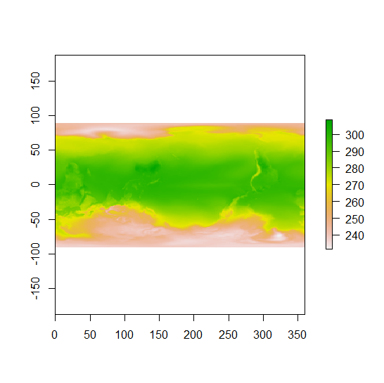
plot(tas.jan1850rGFDL)
plot(tas.jan1851rGFDL)

tas.jan1850rfGFDL <- flip(tas.jan1850rGFDL, direction='y')
tas.jan1851rfGFDL <- flip(tas.jan1851rGFDL, direction='y')

plot(tas.jan1850rfGFDL)
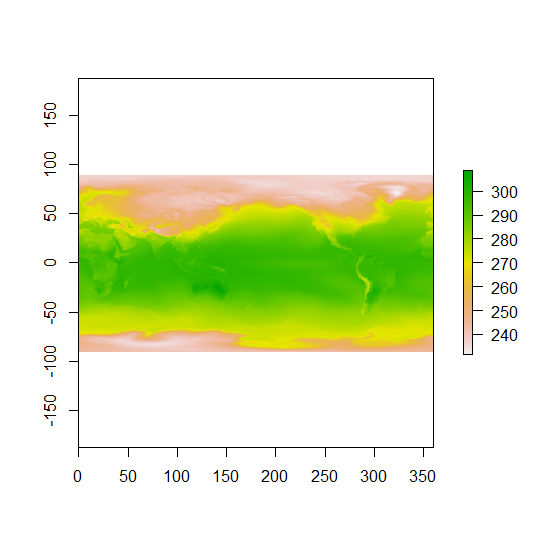
plot(tas.jan1851rfGFDL)

writeRaster(tas.jan1850rfGFDL, "tas.jan1850rfGFDL.tif", "GTiff", overwrite=TRUE)

writeRaster(tas.jan1851rfGFDL, "tas.jan1851rfGFDL.tif", "GTiff", overwrite=TRUE)
Then repeat for each month, each year, each model.
With package ncdfCF you get a more intelligent solution for netCDF files that follow the CF Metadata Conventions (CF), as all CMIP6 files do (among very many other data sets). It is pure R code, no need for external libraries.
Step-by-step
For a single file it works like in the blocks of code below. This is the step-by-step version so that you see and learn what is going on. The compact version for multiple models and variables is further down.
library(ncdfCF)

# Open the netCDF file
(ds <- open_ncdf("~/ts_Amon_GFDL-ESM4_historical_r1i1p1f1_gr1_18500116-19491216.nc"))
#> <Dataset> ts_Amon_GFDL-ESM4_historical_r1i1p1f1_gr1_18500116-19491216
#> Resource   : ~/ts_Amon_GFDL-ESM4_historical_r1i1p1f1_gr1_18500116-19491216.nc
#> Format     : netcdf4
#> Collection : CMIP6
#> Conventions: CF-1.7 CMIP-6.0 UGRID-1.0
#> Keep open  : FALSE
#> Has groups : FALSE
#>
#> Variable:
#>  name long_name           units data_type axes
#>  ts   Surface Temperature K     NC_FLOAT  lon, lat, time
#>
#> External variable: areacella
#>
#> Attributes:
#>  (omitted for brevity)

# Get the data variable `ts`
ts <- ds[["ts"]]

# Summarise the data variable per month over the specific period
(ts_mon <- ts$summarise("ts_mon", mean, "month", 1850:1949))
#> <Data array> ts_mon
#> Long name: Surface Temperature
#>
#> Values: [199.0709 ... 317.926] K
#>     NA: 0 (0.0%)
#>
#> Axes:
#>  axis name long_name length values                                        unit
#>  T    time            12    [1899-01-16T12:00:00 ... 1899-12-16T12:00:00] days since 1850-01-01
#>  X    lon  longitude 288    [0.625 ... 359.375]                           degrees_east
#>  Y    lat  latitude  180    [-89.5 ... 89.5]                              degrees_north
#>
#> Attributes:
#>  name          type     length value
#>  _FillValue    NC_FLOAT  1     1.00000002004088e+20
#>  long_name     NC_CHAR  19     Surface Temperature
#>  units         NC_CHAR   1     K
#>  cell_methods  NC_CHAR  16     area: time: mean
#>  cell_measures NC_CHAR  15     area: areacella
#>  standard_name NC_CHAR  19     surface_temperature
#>  interp_method NC_CHAR  15     conserve_order2
#>  original_name NC_CHAR   2     ts
#>  missing_value NC_FLOAT  1     1.00000002004088e+20
#>  actual_range  NC_FLOAT  2     199.070907, 317.925981

# ts_mon has a "climatological" time axis
ts_mon$axes[["time"]]$time()
#> CF calendar:
#>   Origin  : 1850-01-01T00:00:00
#>   Units   : days
#>   Type    : noleap
#> Climatological time series:
#>   Elements: [1899-01-16T12:00:00 .. 1899-12-16T12:00:00] (average of 30.363636 days between 12 elements)
#>   Period  : month
#>   Years   : 1850 - 1949 (inclusive)
First of all, the file is slightly different than yours, it is GFDL-ESM4 with variable "ts", but that should not make any difference. Some other interesting details:
- The file follows the
CF-1.7metadata conventions. Just the way we like it. - The file has only a single data variable,
tsin this case. CMIP6 files always have only a single data variable, but not every netCDF package will limit itself to just the data variables and show you many more "variables". You can also find the name withnames(ds). - The
summarise()method summarises the variable over time, in this case per month over the years 1850-1949 and using the functionmean(). You could also use other functions, including your own. The result will be aCFArrayinstance with the name "ts_mon". - ts_mon has a climatological axis, meaning that its values are derived via some statistical summary, the
mean()function here. The coordinates it lists are in 1899, midway 1850 and 1949. The boundary values shows the range of dates for each month of the result.
The CFArray instance carefully manages your data, along with useful information such as the axes and its attributes. If you want to get your hands on the actual data you can use the method raw() to get an array with dimensions just as you see it above, T-X-Y with Y values increasing. If you want the classical R ordering, Y-X-T with Y values decreasing, use method array():
arr <- ts_mon$array()
str(arr)
#> num [1:180, 1:288, 1:12] 240 240 240 241 242 ...
#> - attr(*, "dimnames")=List of 3
#>  ..$ lat : chr [1:180] "89.5" "88.5" "87.5" "86.5" ...
#>  ..$ lon : chr [1:288] "0.625" "1.875" "3.125" "4.375" ...
#>  ..$ time: chr [1:12] "1899-01-16T12:00:00" "1899-02-15T00:00:00" "1899-03-16T12:00:00" "1899-04-16T00:00:00" ...
Easy! That's 12,000 lines of your code done.
In a function
Putting it all in a function is probably the best way to code once, run often. You can then also add further processing or other tweaks to simplify your analysis.
processCMIP6model <- function(fn, name, FUN) {
  ds <- open_ncdf(fn)
  var <- ds[[names(ds)]]
  var$summarise(name, FUN, "month", 1850:1949)
}
Assuming your 6 CMIP6 models are in a single directory you can do it all in one sweep:
lf <- list.files("~/CMIP6/data/directory", ".nc$", full.names = TRUE)
res <- lapply(lf, processCMIP6model, "ts_mon", mean)
names(res) <- basename(lf)
res is a list with one element for each of the files in your directory. Note that you can do this with as many CMIP6 files as you have, mixing variables and functions as you go.
Plotting and other analyses
You can easily plot the resulting list using the terra package (which is the successor to the raster package):
# Starting with the list of model results from above, or use an individual CFArray
model1r <- terra::rast(res[[1]])
# Optionally, set layer names
names(model1r) <- month.abb
model1r
#> class : SpatRaster
#> dimensions : 180, 288, 12 (nrow, ncol, nlyr)
#> resolution : 1, 1 (x, y)
#> extent : 0, 288, 0, 180 (xmin, xmax, ymin, ymax)
#> coord. ref. :
#> source(s) : memory
#> names : Jan, Feb, Mar, Apr, May, Jun, ...
#> min values : 228.2004, 221.2835, 208.5045, 202.0122, 200.8219, 200.0914, ...
#> max values : 313.0564, 310.6226, 311.3170, 311.8899, 313.6404, 317.6213, ...
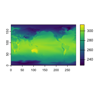
plot(model1r, "Jan")
Other kinds of analysis can similarly be done directly using the array in the res list.
72,000 lines of code done.
- How to find correct projection of the shapefile data for leaflet map in r?
- How to use regex in R to shorten strings by one space
- R CRAN Check fail when using parallel functions
- Replacing several rows of data in a column efficiently using condition in a pipeline
- Iterate over vectors from an imported dataframe row-wise
- Split the legend into three rows with headings for a nested facet_wrap
- Why replace works with a boolean mask?
- Not able properly rasterize polygon dataset using terra::rasterize()
- Less than symbol ("<") in cloze schoice in Canvas (html select dropdown) shows as &lt;
- R/exams docx output does not include images
- How to have primitive discard additional arguments
- Functions Causing Objects to Disappear
- How to repel texts equidistantly on a secondary y-axis of a facet_grid?
- How can I add some text to a ggplot2 graph in R outside the plot area?
- Extracting Exact p-values from the "did" Package Output in R
- How can I set column types of several columns in empty R data frame?
- Adjust vertical line based on maximum value in graph plotly
- Combining Two Dataframes Based on Multiple Conditions & Removing Rows that Don't Match
- independent sample t-test in R using test statistics (mean, std. dev, count)
- How do I load a package without installing it in R?
- survcheck: 'x' must be an array of at least two dimensions
- Insert variable names and their specific values between the last column of facets and the strips of a facet_grid in R
- Use a recorded plot for officer
- Errors when using RStudio's Git tools
- Orientation of an irregular window changes the distance r over which secondary summary statistics are estimated
- Elegant way to check for missing packages and install them?
- How to create tmap labels along lines with rotated crs?
- How to access the value of a reactive output inside the browser console with jQuery?
- Convert excel column names to numbers
- How to adjust a node width in a Sankey plot in R?