How to Highlight the Difference Between Two Bar Charts in MATLAB?
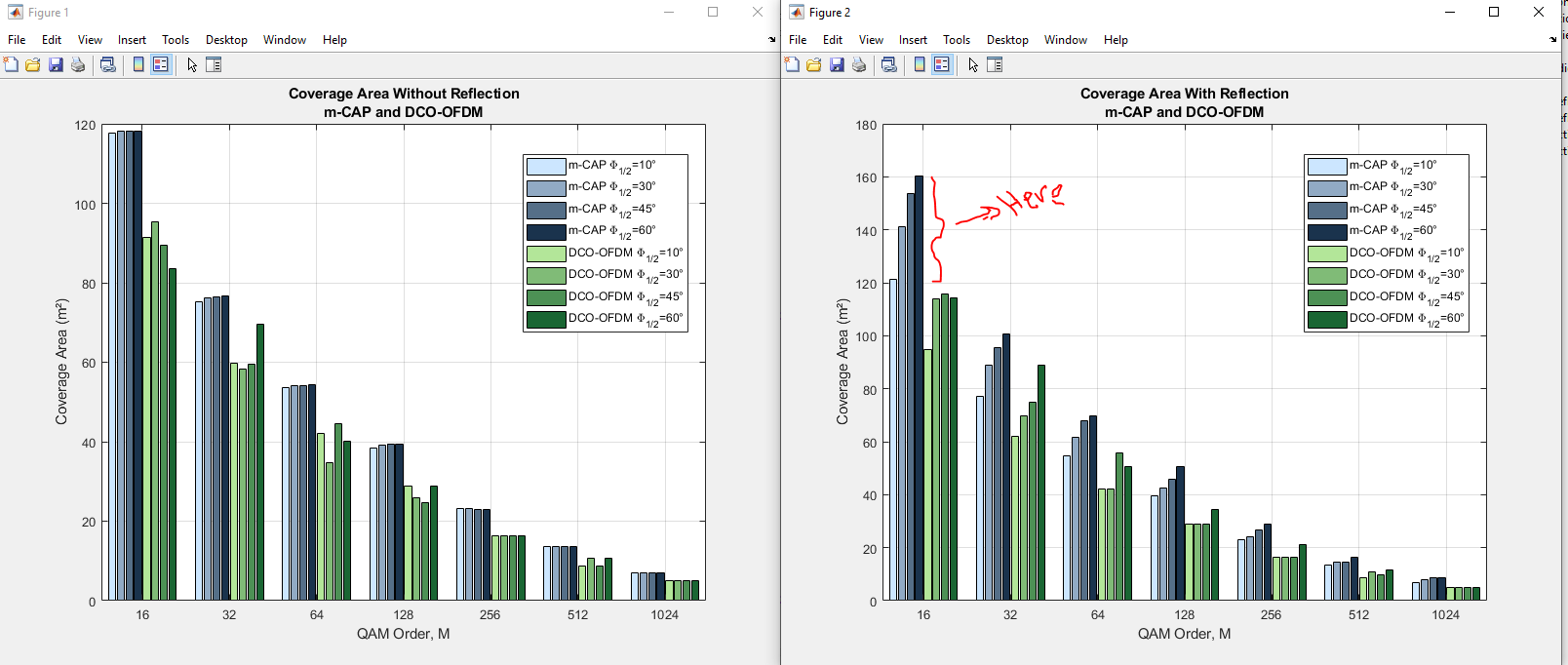
I am working on a MATLAB project where I have two sets of data:
1- "No Reflection": Represents baseline coverage area values. 2- "With Reflection": Represents coverage area values with an additional reflection effect.
I am plotting these two datasets as a grouped bar chart and I want to highlight the difference caused by the reflection. Specifically, I need the section of each bar corresponding to the difference (reflection effect) to be highlighted in a different color on top of the "No Reflection" bars.
Example: For instance, if:
- "No Reflection" value for the first bar (QAM = 16) is 120 m².
- "With Reflection" value for the same bar is 160 m².
I want to:
1- Plot a bar representing 120 m² (base value for "No Reflection").
2- Highlight the difference (160 - 120 = 40 m²) on top of the blue bar in red (highlight for the reflection effect).
I want to apply this on all the bars on the image that is on the right side. Any assistance, please?
This is my code:
close all;
clear variables;
clc;

QAM = [16, 32, 64, 128, 256, 512, 1024];

%% m_CAP modulation

% Beamsteering without reflection
VEC_Beam_no_reflection_mCAP = [
    117.5491   75.1933   53.5396   38.3105   23.0815   13.5634    6.9007; % Theta = 10
    118.2629   76.1452   54.0155   39.0244   23.0815   13.5634    6.9007; % Theta = 30
    118.2629   76.3831   54.0155   39.5003   22.8435   13.5634    6.9007; % Theta = 45
    118.2629   76.6211   54.2534   39.5003   22.8435   13.5634    6.9007  % Theta = 60
];

% Beamsteering with reflection
VEC_Beam_reflection_mCAP = [
    121.3563   77.0970   54.7293   39.7383   22.8435   13.5634    6.9007; % Theta = 10
    141.1065   88.7567   61.6300   42.5937   24.2713   14.5152    7.8525; % Theta = 30
    153.7180   95.6573   67.8168   45.6871   26.6508   14.5152    8.8043; % Theta = 45
    160.3807  100.6544   69.7204   50.4462   28.7924   16.4188    8.8043  % Theta = 60
];

%% DCO-OFDM modulation

% Beamsteering without reflection
VEC_Beam_no_reflection_OFDM = [
    91.3742   59.7264   42.1178   28.7924   16.4188    8.8043    4.9970; % Theta = 10
    95.4194   58.2986   34.7412   25.9369   16.4188   10.7079    4.9970; % Theta = 30
    89.4706   59.4884   44.4973   24.7472   16.4188    8.8043    4.9970; % Theta = 45
    83.5217   69.4825   40.2142   28.7924   16.4188   10.7079    4.9970  % Theta = 60
];

% Beamsteering with reflection
VEC_Beam_reflection_OFDM = [
    94.7055   61.8679   42.1178   28.7924   16.4188    8.8043    4.9970; % Theta = 10
    113.9798   69.7204   42.1178   28.7924   16.4188   10.7079    4.9970; % Theta = 30
    115.6454   74.9554   55.6811   28.7924   16.4188    9.7561    4.9970; % Theta = 45
    114.4557   88.7567   50.6841   34.5033   21.1779   11.6597    4.9970  % Theta = 60
];

%% Combine Data for Bar Chart
angles = [10, 30, 45, 60];
data_no_reflection = [VEC_Beam_no_reflection_mCAP; VEC_Beam_no_reflection_OFDM];
data_with_reflection = [VEC_Beam_reflection_mCAP; VEC_Beam_reflection_OFDM];

% Generate gradient colors for m-CAP (blue) and DCO-OFDM (green)
mCAP_blue_gradient = [linspace(0.8, 0.1, 4)', linspace(0.9, 0.2, 4)', linspace(1.0, 0.3, 4)']; % Light to dark blue
DCO_green_gradient = [linspace(0.7, 0.1, 4)', linspace(0.9, 0.4, 4)', linspace(0.6, 0.2, 4)']; % Light to dark green

% Combine colors
custom_colors = [mCAP_blue_gradient; DCO_green_gradient];

% Plot for No Reflection
figure('Position', [100, 100, 800, 600]);
b1 = bar(data_no_reflection', 'grouped');
for k = 1:length(b1)
    b1(k).FaceColor = 'flat';
    b1(k).CData = repmat(custom_colors(k, :), size(b1(k).CData, 1), 1);
end
xticks(1:length(QAM));
xticklabels(string(QAM));
xlabel('QAM Order, M');
ylabel('Coverage Area (m²)');
title({'Coverage Area Without Reflection', 'm-CAP and DCO-OFDM'});
legend(["m-CAP \Phi_{1/2}=10°", "m-CAP \Phi_{1/2}=30°", "m-CAP \Phi_{1/2}=45°", "m-CAP \Phi_{1/2}=60°", ...
        "DCO-OFDM \Phi_{1/2}=10°", "DCO-OFDM \Phi_{1/2}=30°", "DCO-OFDM \Phi_{1/2}=45°", "DCO-OFDM \Phi_{1/2}=60°"], ...
       'Location', 'Best');
grid on;

% Plot for With Reflection
figure('Position', [100, 100, 800, 600]);
b2 = bar(data_with_reflection', 'grouped');
for k = 1:length(b2)
    b2(k).FaceColor = 'flat';
    b2(k).CData = repmat(custom_colors(k, :), size(b2(k).CData, 1), 1);
end
xticks(1:length(QAM));
xticklabels(string(QAM));
xlabel('QAM Order, M');
ylabel('Coverage Area (m²)');
title({'Coverage Area With Reflection', 'm-CAP and DCO-OFDM'});
legend(["m-CAP \Phi_{1/2}=10°", "m-CAP \Phi_{1/2}=30°", "m-CAP \Phi_{1/2}=45°", "m-CAP \Phi_{1/2}=60°", ...
        "DCO-OFDM \Phi_{1/2}=10°", "DCO-OFDM \Phi_{1/2}=30°", "DCO-OFDM \Phi_{1/2}=45°", "DCO-OFDM \Phi_{1/2}=60°"], ...
       'Location', 'Best');
grid on;
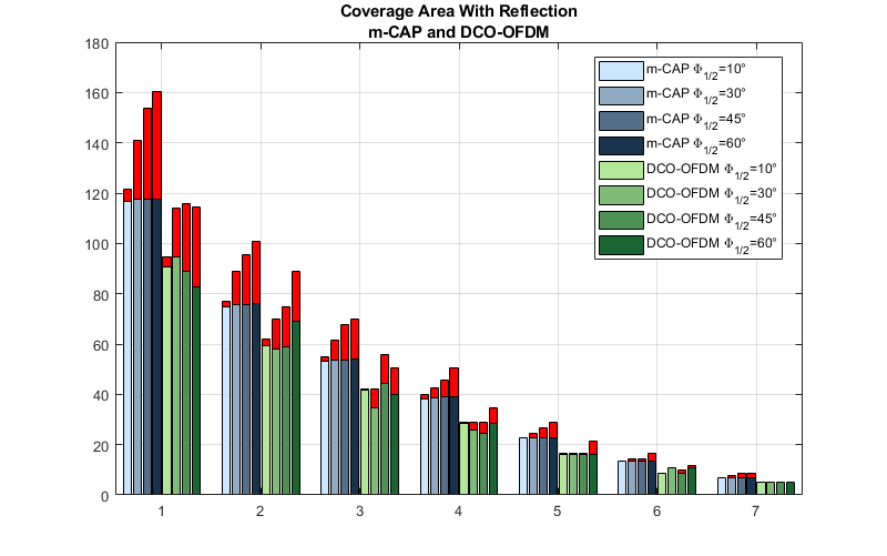
If you weren't creating a grouped barchart you could make these as stacked bars instead, with the top part of the stack equal to the difference between the two.
Since you are using a grouped chart, a simple approach would be to plot the taller bars first (with the whole bar red), then hold on and plot the shorter bars.
You can set the HandleVisibility to off for the red bars so that they don't appear in the legend.
It would look something like this from your example:
f = figure('Position', [100, 100, 800, 600]);

% Set "HandleVisibility" to off so these bars don't appear in legend
b2 = bar(data_with_reflection', 'grouped','HandleVisibility','off');
for k = 1:length(b2)
    b2(k).FaceColor = 'flat';
    b2(k).CData = repmat([1,0,0], size(b2(k).CData, 1), 1); % [1,0,0] for red bars
end

% Plot for No Reflection
hold on; % To plot 2nd set of bars on top

b1 = bar(data_no_reflection', 'grouped');
for k = 1:length(b1)
    b1(k).FaceColor = 'flat';
    b1(k).CData = repmat(custom_colors(k, :), size(b1(k).CData, 1), 1);
end

grid on;
xticks(1:length(QAM));
xticklabels(string(QAM));
title({'Coverage Area With Reflection', 'm-CAP and DCO-OFDM'});
legend(["m-CAP \Phi_{1/2}=10°", "m-CAP \Phi_{1/2}=30°", "m-CAP \Phi_{1/2}=45°", "m-CAP \Phi_{1/2}=60°", ...
        "DCO-OFDM \Phi_{1/2}=10°", "DCO-OFDM \Phi_{1/2}=30°", "DCO-OFDM \Phi_{1/2}=45°", "DCO-OFDM \Phi_{1/2}=60°"], ...
       'Location', 'Best');
Output:
- Why is im2col more efficient than naive 2d convolution?
- Concatenating empty array in Numpy
- Why doesn't Matlabs Isosurface work here?
- Save exact image output from imagesc in matlab
- How to change the order of lines in a Matlab figure?
- What is the difference between .m and .mat files in MATLAB
- How to add a legend without plot rescaling?
- Is there a more elegant way to write sum in MATLAB code
- Plotting arrays using a grouped horizontal bar graph
- Coloring Triangulation from Set of Points
- Matlab image features extraction error (ifcb-analysis)
- How to zoom in/out in Matlab editor?
- 1D Poisson equation in MATLAB
- How to implement delta E color difference method of an image in matlab?
- Plotting a function inside a polygon in MATLAB
- Is there a way to make an anonymous function without output?
- Matlab function for lorentzian fit with global variables
- Error forming mini-batch for network input
- Constraining parameters using mldivide
- Pyramidal Histogram Of Oriented Gradients - Trilinear interpolation
- How to know the size of a variable in MATLAB
- How to get the next higher power of 2?
- Unable to understand product of Sinusoid signal with Hann window function in MATLAB R2024b
- List of all built-in symbols in Matlab/Octave
- Handling large number of name/value parameters in MATLAB
- Infusion-pump Model- PID-controller- running very slow
- What is contained in the "function workspace" field in .mat file?
- `numpy.testing.assert_array_equal` fails when comparing structured numpy arrays with array fields
- MATLAB reports "Exception in thread "AWT-EventQueue-0" java.lang.NullPointerException"
- Proper way to add noise to signal

