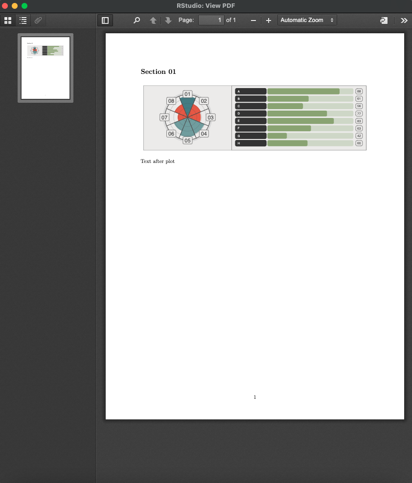
grid.arrange's relative height argument didn't works well in RMarkdown

Preamble

I have 2 plots in ggplot2 and want to put them in RMarkdown document. I'm mainly using grid.arrange to do that. But since those plots have completely different heights, I need to adjust using heights = c(0.7, 1)

Problem

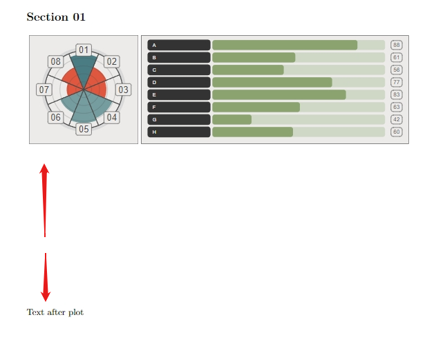
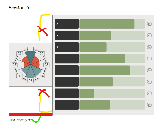
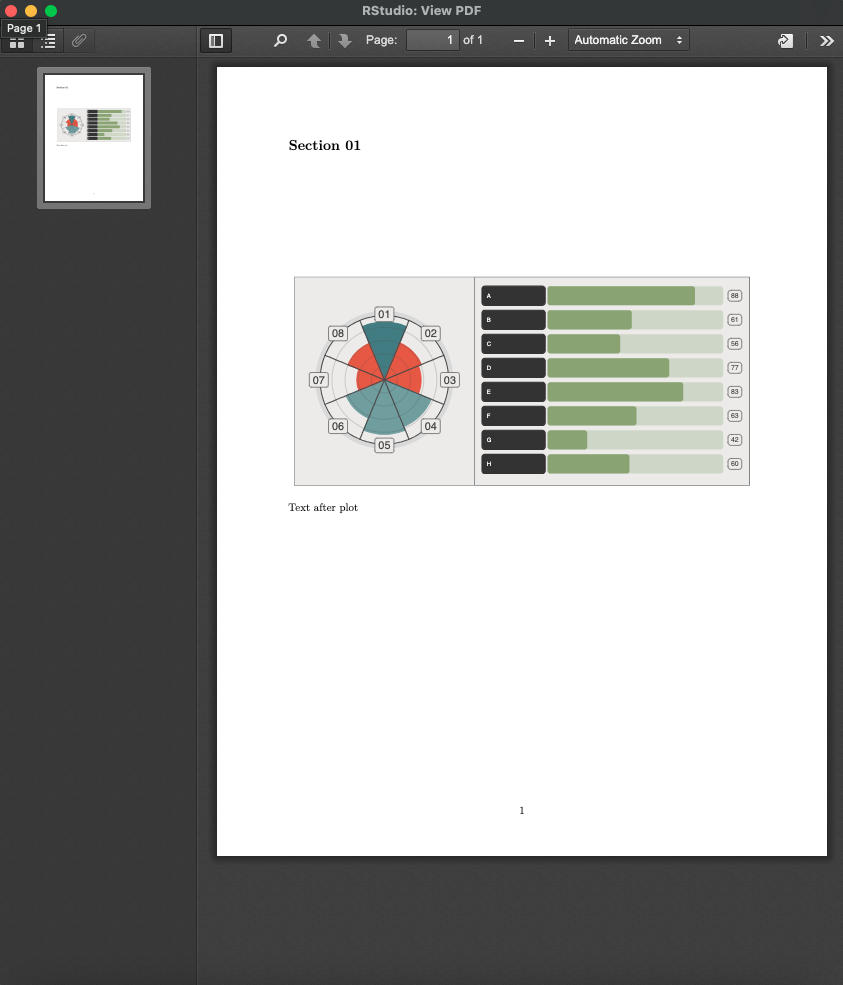
Adjusting the heights left a lot of empty space in the document

Goal

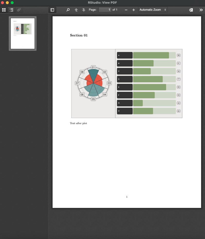
I want to integrate (put) those plots side-by-side with a tidy manner, without huge space separating the combined plots and the text after.

Code

---
title: ""
output: pdf_document
geometry: 
  - margin=1in
  - headheight=14pt
fontsize: 11pt

---

\noindent

\\```{r setup, include=FALSE, cache=FALSE}
knitr::opts_chunk$set(
  fig.path = '',      # No separate figure folders
  echo = FALSE,          # Show code chunks
  warning = FALSE,      # Suppress warnings
  message = FALSE       # Suppress messages
)
\\```

\section{Section 01}

\\```{r plot_data, cache=TRUE}
# Create data frame
data <- data.frame(
  labels = c(LETTERS[1:8]),
  values = c(88, 61, 56, 77, 83, 63, 42, 60)
)
\\```


\\```{r plotgrid, dependson="plot_data", fig.cap=NULL}
library(tidyverse)

data_nude_bar <- as.tibble(data)

data_nude_bar <- data_nude_bar %>%
  mutate(
    num = rev(row_number()),
    store_lower = 25,
    store_upper = values,
    text_bg_col = "white",
    text_bg_outline = "grey20"
  ) 

# Create the chart

bar_height <- 0.4

p_bar <- ggplot(data_nude_bar) +
  ggchicklet::geom_rrect(
    # mid rec base
    aes(
      xmin = store_lower, xmax = 100, 
      ymin = num - bar_height, ymax = num + bar_height,
      fill = "#b9c7a8", alpha = .5
    ),
    radius = grid::unit(1, "mm")
  ) +
  ggchicklet::geom_rrect(
    # mid rec fill
    aes(
      xmin = store_lower, xmax = store_upper, 
      ymin = num - bar_height, ymax = num + bar_height,
      fill = "#8ca470"
    ),
    radius = grid::unit(1, "mm")
  ) +
  ggchicklet::geom_rrect(
    # left rec
    aes(
      xmin = -3, xmax = 24,
      ymin = num - bar_height, ymax = num + bar_height,
      fill = "gray20", colour = text_bg_outline
    ),
    radius = grid::unit(1, "mm")
  ) +
  scale_fill_identity() +
  scale_color_identity() +
  geom_text(
    # trait name
    aes(
      label = labels, x = -1, y = num,
      hjust = 0, color = "white"
    ),
    size = 2
  ) +
  geom_label(
    aes(label = values,x = 105, y = num),
    hjust = 0.5, size = 2.5, label.padding = unit(3, "pt"),
    color = "grey30", fill = "#edecea",
    label.r = unit(3, "pt")
  ) +
  coord_cartesian(clip = "off", xlim = c(0, 100)) +
  theme_minimal() +
  theme(
    plot.margin = margin(r = 15, unit = "pt"),
    legend.position = "none",
    panel.grid = element_blank(),
    axis.text = element_blank(),
    axis.title = element_blank(),
    plot.background = element_rect(
      color = "grey30",
      fill = "#edecea"
    )
  )


data_circular_bar <- as.tibble(data) %>%
  mutate(
    bar_color = case_when(
      values < 62 ~ "#de583f",
      values < 85 ~ "#759d9f",
      values >= 85 ~ "#4b7d84"
    ),
    labels = factor(labels, levels = labels),
    labelnum = factor(
      c("01", "02", "03", "04", "05", "06", "07", "08"),
      levels = c("01", "02", "03", "04", "05", "06", "07", "08")
    )
  )


scaling_factor <- max(100)

p_circular <- ggplot(data_circular_bar %>% mutate(values = values / scaling_factor), 
       aes(labels, values, fill = bar_color)) +
  geom_col(width = 1, aes(color = after_scale(fill))) +
  annotate("linerange", ymin = 0, ymax = 1.02, x = seq(nrow(data)) - 0.5,
           color = "#494949") +
  geom_hline(yintercept = c(0, 2, 4, 6, 8) / 10, color = "#494949", alpha = 0.2) +
  geom_hline(yintercept = 1.02, color = "#d9d9d9", linewidth = 2) +
  geom_hline(yintercept = .98, color = "#494949") +
  geom_label(aes(y = 1, label = labelnum), fill = "#edecea", color = "#494949",
             size = 4) +
  scale_fill_identity() +
  coord_polar(start = -pi/8) +
  theme_void() +
  scale_y_continuous(limits = c(0, 1.1), expand = c(0, 0)) +
  theme(plot.background = element_rect(fill = "#edecea", color = "grey30"))

library(gridExtra)
library(grid)
grid.arrange(p_circular, p_bar, ncol = 2, heights = c(.7,1), widths = c(3,7))




\\```

Text after plot

Effort so far

1. Using \vspace{-20pt} right after the plot: didn't work, result still the same
2. Removing heights argument makes the space disappear, but the height of the plots become their original, and it looks bad

3. using patchwork also still have exact same problem

Based on that all, I need help to put those plots side by side without leaving a lot of empty space

With patchwork you can specify the height of a 'blank' (#), e.g.

library(patchwork)
p_circular + p_bar + plot_layout(heights = c(0.5, 1), widths = c(0.7, 1),
                                 nrow = 1,
                                 design = "##
                                           AB")

library(patchwork)
p_circular + p_bar + plot_layout(heights = c(0.1, 1), widths = c(0.7, 1),
                                 nrow = 1,
                                 design = "##
                                           AB")

Combine that with fig.height in the rmarkdown header, and you should be able to solve your problem, e.g.

```{r plotgrid, dependson="plot_data", fig.cap=NULL, fig.height=2}

...

library(patchwork)
p_circular + p_bar + plot_layout(heights = c(0.5, -0.05), widths = c(0.7, 1),
                                 nrow = 1,
                                 design = "AB
                                           ##")

Also, I've just remembered your reply from Friday (https://stackoverflow.com/a/79277334/12957340) - I'll edit that answer now to make it more fit-for-purpose.